vlookup to cross reference lists

1. How do I do a Vlookup to compare two lists?
2. How do you cross reference a list in Excel?
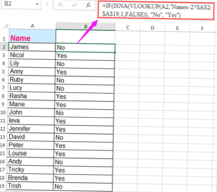
3. How do I do a Vlookup in Excel to compare two columns?
4. What does cross reference mean?
5. What is the easiest way to cross reference in Excel?
6. What is the correct Vlookup formula?
7. How use Vlookup step by step?
8. How do I compare two Excel lists for differences?
9. How do you cross reference two lists in sheets?
10. What are the 3 types of cell references in Excel?
11. How do I get a list of names in Excel?

How do I do a Vlookup to compare two lists?

Compare Two Lists and Highlight Missing Records

1. Select all the cells of the table except the header row.
2. Click Conditional Formatting on the Home tab of the Ribbon and select New Rule.
3. Select Use a Formula to determine which cells to format from the top half of the window.

How do you cross reference a list in Excel?

A Ridiculously easy and fun way to compare 2 lists

1. Select cells in both lists (select first list, then hold CTRL key and then select the second)
2. Go to Conditional Formatting > Highlight Cells Rules > Duplicate Values.
3. Press ok.
4. There is nothing do here. Go out and play!

How do I do a Vlookup in Excel to compare two columns?

How to Compare Two Columns in Excel

1. Click the Compare two columns worksheet tab in the VLOOKUP Advanced Sample file. ...
2. Add columns in your workbook so you have space for results. ...
3. Type the first VLOOKUP formula in cell E2: ...
4. Click Enter on your keyboard and drag the VLOOKUP formula down through cell C17.

What does cross reference mean?

(Entry 1 of 2) : a notation or direction at one place (as in a book or filing system) to pertinent information at another place.

What is the easiest way to cross reference in Excel?

However, it is easier and more reliable to let Excel write the reference for you. Type an equal sign (=) into a cell, click on the Sheet tab, and then click the cell that you want to cross-reference. As you do this, Excel writes the reference for you in the Formula Bar. Press Enter to complete the formula.

What is the correct Vlookup formula?

In its simplest form, the VLOOKUP function says: =VLOOKUP(What you want to look up, where you want to look for it, the column number in the range containing the value to return, return an Approximate or Exact match – indicated as 1/TRUE, or 0/FALSE).

How use Vlookup step by step?

How to use VLOOKUP in Excel

1. Step 1: Organize the data. ...
2. Step 2: Tell the function what to lookup. ...
3. Step 3: Tell the function where to look. ...
4. Step 4: Tell Excel what column to output the data from. ...
5. Step 5: Exact or approximate match.

How do I compare two Excel lists for differences?

Compare Two Columns and Highlight Matches

1. Select the entire data set.
2. Click the Home tab.
3. In the Styles group, click on the 'Conditional Formatting' option.
4. Hover the cursor on the Highlight Cell Rules option.
5. Click on Duplicate Values.
6. In the Duplicate Values dialog box, make sure 'Duplicate' is selected.

How do you cross reference two lists in sheets?

Using Power Tools to compare columns

1. Once Power Tools is added to your Google Sheets, go to the Add-Ons pull-down menu.
2. Select Power Tools.
3. Then select Start.
4. Click the 'Data' menu option then select 'Compare two sheets'
5. Enter the ranges of the columns you want to compare.

What are the 3 types of cell references in Excel?

Now there are three kinds of cell references that you can use in Excel:

• Relative Cell References.
• Absolute Cell References.
• Mixed Cell References.

How do I get a list of names in Excel?

You can find a named range by using the Go To feature—which navigates to any named range throughout the entire workbook.

1. You can find a named range by going to the Home tab, clicking Find & Select, and then Go To. Or, press Ctrl+G on your keyboard.
2. In the Go to box, double-click the named range you want to find.