A Ridiculously easy and fun way to compare 2 lists
- Select cells in both lists (select first list, then hold CTRL key and then select the second)
- Go to Conditional Formatting > Highlight Cells Rules > Duplicate Values.
- Press ok.
- There is nothing do here. Go out and play!
- How do you cross reference two sets of data in Excel?
- How do I compare two lists in Excel for matches?
- How do I compare list names in Excel?
- How do you compare two lists?
- How do you create a dynamic cell reference in Excel?
- How do you cross reference two lists in sheets?
- How use Vlookup step by step?
- How do I check if a name is in a list in Excel?
- Can Excel cross check two lists?
- How do you name a list in Excel?
- Can you compare Excel documents?
How do you cross reference two sets of data in Excel?
You can refer to cells of another workbook using the same method. Just be sure that you have the other Excel file open before you begin typing the formula. Type an equal sign (=), switch to the other file, and then click the cell in that file you want to reference. Press Enter when you're done.
How do I compare two lists in Excel for matches?
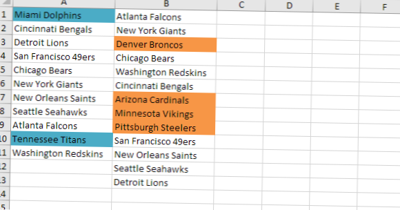
Compare Two Columns and Highlight Matches
- Select the entire data set.
- Click the Home tab.
- In the Styles group, click on the 'Conditional Formatting' option.
- Hover the cursor on the Highlight Cell Rules option.
- Click on Duplicate Values.
- In the Duplicate Values dialog box, make sure 'Duplicate' is selected.
How do I compare list names in Excel?
Compare Two Lists
- First, select the range A1:A18 and name it firstList, select the range B1:B20 and name it secondList.
- Next, select the range A1:A18.
- On the Home tab, in the Styles group, click Conditional Formatting.
- Click New Rule.
- Select 'Use a formula to determine which cells to format'.
- Enter the formula =COUNTIF(secondList,A1)=0.
How do you compare two lists?
The methods of comparing two lists are given below.
- The cmp() function.
- The set() function and == operator.
- The sort() function and == operator.
- The collection.counter() function.
- The reduce() and map() function.
How do you create a dynamic cell reference in Excel?
To create an Excel dynamic reference to any of the above named ranges, just enter its name in some cell, say G1, and refer to that cell from an Indirect formula =INDIRECT(G1) .
How do you cross reference two lists in sheets?
Using Power Tools to compare columns
- Once Power Tools is added to your Google Sheets, go to the Add-Ons pull-down menu.
- Select Power Tools.
- Then select Start.
- Click the 'Data' menu option then select 'Compare two sheets'
- Enter the ranges of the columns you want to compare.
How use Vlookup step by step?
How to use VLOOKUP in Excel
- Step 1: Organize the data. ...
- Step 2: Tell the function what to lookup. ...
- Step 3: Tell the function where to look. ...
- Step 4: Tell Excel what column to output the data from. ...
- Step 5: Exact or approximate match.
How do I check if a name is in a list in Excel?
Besides the Find and Replace function, you can use a formula to check if a value is in a list. Select a blank cell, here is C2, and type this formula =IF(ISNUMBER(MATCH(B2,A:A,0)),1,0) into it, and press Enter key to get the result, and if it displays 1, indicates the value is in the list, and if 0, that is not exist.
Can Excel cross check two lists?
The quickest way to find all about two lists is to select them both and them click on Conditional Formatting -> Highlight cells rules -> Duplicate Values (Excel 2007). The result is that it highlights in both lists the values that ARE the same.
How do you name a list in Excel?
How to Create Named Ranges in Excel
- Select the range for which you want to create a Named Range in Excel.
- Go to Formulas –> Define Name.
- In the New Name dialogue box, type the Name you wish to assign to the selected data range. ...
- Click OK.
Can you compare Excel documents?
If you have two workbooks open in Excel that you want to compare, you can run Spreadsheet Compare by using the Compare Files command.