How To Customize The Chart Legend In MS Office

Click the chart, and then click the Chart Layout tab. To change the position of the legend, under Labels, click Legend, and then click the legend position that you want. To change the format of the legend, under Labels, click Legend, click Legend Options, and then make the format changes that you want.

1. How do I change the legend in an Excel chart?
2. How do you show the legend in Excel chart?
3. How do I change the axis and legend in Excel?
4. How do you customize a chart?
5. What is legend in Excel chart?
6. How do you create a legend in Excel?
7. Is a legend the same as a key?
8. What is a legend on a chart?
9. How do you separate a chart legend in Excel?
10. How do I switch axis titles in Excel?
11. How do I switch rows and columns in Excel?
12. How do I change the axis scale in Excel 2020?

How do I change the legend in an Excel chart?

1. Select your chart in Excel, and click Design > Select Data.
2. Click on the legend name you want to change in the Select Data Source dialog box, and click Edit. ...
3. Type a legend name into the Series name text box, and click OK.

How do you show the legend in Excel chart?

Add a chart legend

1. Click the chart.
2. Click Chart Elements. next to the table.
3. Select the Legend check box. The chart now has a visible legend.

How do I change the axis and legend in Excel?

Change the way that data is plotted

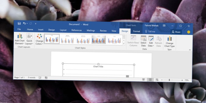
1. Click anywhere in the chart that contains the data series that you want to plot on different axes. This displays the Chart Tools, adding the Design, Layout, and Format tabs.
2. On the Design tab, in the Data group, click Switch Row/Column.

How do you customize a chart?

Select the chart and go to the Chart Tools tabs (Design and Format) on the Excel ribbon. Right-click the chart element you would like to customize, and choose the corresponding item from the context menu. Use the chart customization buttons that appear in the top right corner of your Excel graph when you click on it.

What is legend in Excel chart?

A Legend is a representation of legend keys or entries on the plotted area of chart or graph which are linked to the data table of the chart or graph. By default, it may show in the bottom or right side of the chart. The data in a chart is organized with the combination of Series and Categories.

How do you create a legend in Excel?

Click the chart, and then click the Chart Design tab. Click Add Chart Element > Legend. To change the position of the legend, choose Right, Top, Left, or Bottom. To change the format of the legend, click More Legend Options, and then make the format changes that you want.

Is a legend the same as a key?

A key or legend is a box that lists the symbols that are used on a map. It also explains what each symbol means. “Key” and “legend” are two names for the same thing.

What is a legend on a chart?

The legend is a side section of the chart that gives a small text description of each series. You can specify the text associated with each series in this legend, and specify where on the chart it should appear.

How do you separate a chart legend in Excel?

Tested in Excel 2010:

1. Select your chart.
2. From the Ribbon tool select Copy as Picture... (Click the drop down next to Copy)
3. Paste your picture (a copy of the entire chart)
4. Right click somewhere on the picture. ...
5. Drag the crop markers to remove the unwanted area around your legend.

How do I switch axis titles in Excel?

Drag a title to the location that you want

1. In the chart, click the title that you want to move to another location.
2. To move the title, position the pointer on the border of the title box so that it changes to a four-headed arrow. , and then drag the title box to the location that you want.

How do I switch rows and columns in Excel?

Transpose (rotate) data from rows to columns or vice versa

1. Select the range of data you want to rearrange, including any row or column labels, and press Ctrl+C. ...
2. Choose a new location in the worksheet where you want to paste the transposed table, ensuring that there is plenty of room to paste your data.

How do I change the axis scale in Excel 2020?

Figure 1.

1. Right-click on the axis whose scale you want to change. Excel displays a Context menu for the axis.
2. Choose Format Axis from the Context menu. ...
3. Make sure Axis Options area is expanded. ...
4. Adjust the Bounds and Units settings, as desired. ...
5. Close the Format Axis task pane.