How to Create Sparklines in Excel 2016

1. How do I create a Sparkline in Excel?
2. How do I activate Sparklines in Excel 2016?
3. What are sparklines compared to in Excel 2016?
4. How do you insert a row in Excel 2016?
5. How do you create a heatmap in Excel?
6. How do you create scenarios in Excel?
7. How do I enable filtering in Excel?
8. What are the three types of sparklines in Excel?
9. How do I enable Sparklines in Excel 2007?
10. How do you switch rows and columns in Excel?
11. How do I show a bar chart in Excel cell?
12. Which formula is not equivalent to all of the other?

How do I create a Sparkline in Excel?

How to Create Sparklines in Excel

1. Create a table in an excel sheet.
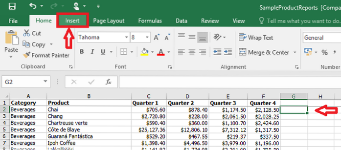
2. Click on the cell G2 in which you want the sparkline and go to Insert tab.
3. In the Sparklines Group click on 'Line'.
4. 'Create Sparklines' Dialog box appears.
5. Now in Data Range select range B2: F2 from row.
6. Now click OK & you will get Sparklines in excel.

How do I activate Sparklines in Excel 2016?

To create your first set of Sparklines in Excel:

1. Select a range of numbers that you'd like to present in Sparklines form, as shown in Figure 2.
2. Choose Insert, and then pick one of the Sparklines options.
3. Specify a Location Range within the Create Sparklines dialog box, and then click OK.

What are sparklines compared to in Excel 2016?

Sparklines are tiny graphs generally about the size of the text that surrounds them. In Excel 2016, sparklines are the height of the worksheet cells whose data they represent and can be any of the following chart types: Line that represents the relative value of the selected worksheet data.

How do you insert a row in Excel 2016?

MS Excel 2016: Insert a new row

1. Right-click and select "Insert" from the popup menu.
2. When the Insert window appears, select the "Entire row" option and click on the OK button.
3. A new row should now be inserted above your current position in the sheet. ...
4. NEXT.

How do you create a heatmap in Excel?

1. Step 1: Enter data. Enter the necessary data in a new sheet. ...
2. Step 2: Select the data. Select the dataset for which you want to generate a heatmap. ...
3. Step 3: Use conditional formatting. If you are using Excel, go to “Home”, click on “Conditional Formatting”, and select “Color Scales”. ...
4. Step 4: Select the color scale.

How do you create scenarios in Excel?

Create the First Excel Scenario

1. On the Ribbon's Data tab, click What If Analysis.
2. Click Scenario Manager.
3. In the Scenario Manager, click the Add button.
4. Type name for the Scenario. ...
5. Press the Tab key, to move to the Changing cells box.
6. On the worksheet, select cells B1.
7. Hold the Ctrl key, and select cells B3:B4.

How do I enable filtering in Excel?

How?

1. On the Data tab, in the Sort & Filter group, click Filter.
2. Click the arrow. in the column header to display a list in which you can make filter choices. Note Depending on the type of data in the column, Microsoft Excel displays either Number Filters or Text Filters in the list.

What are the three types of sparklines in Excel?

There are three different types of sparklines: Line, Column, and Win/Loss. Line and Column work the same as line and column charts. Win/Loss is similar to Column, except it only shows whether each value is positive or negative instead of how high or low the values are.

How do I enable Sparklines in Excel 2007?

Making Sparklines

1. Step 1: Highlight cells B4 through M4 and click the Insert tab. ...
2. Step 2: Click the Line option and select the 2D line chart, which is the first option.
3. Step 3: Click the legend and press the delete key.
4. Step 4: Click the horizontal axis and press the delete key.

How do you switch rows and columns in Excel?

Transpose (rotate) data from rows to columns or vice versa

1. Select the range of data you want to rearrange, including any row or column labels, and press Ctrl+C. ...
2. Choose a new location in the worksheet where you want to paste the transposed table, ensuring that there is plenty of room to paste your data.

How do I show a bar chart in Excel cell?

This method will guide you to insert an in-cell bar chart with the Data Bars of Conditional Formatting feature in Excel. Please do as follows: 1. Select the column you will create in-cell bar chart based on, and click Home > Conditional Formatting > Data Bars > More Rules.

Which formula is not equivalent to all of the other?

In Excel, <> means not equal to. The <> operator in Excel checks if two values are not equal to each other.