- Where is the chart filters button in Excel?
- How do I turn on the filter button in Excel?
- Where is the chart filters button in Excel Mac?
- Why is filter button greyed out in Excel?
- How do you expand the range of a chart in Excel?
- How do I fill a shape in an Excel chart?
- How do you hide filter buttons on a table?
- Why can't I sort my Excel spreadsheet?
- How do I enable filters in Excel 2016?
- How do I reverse the order of categories in Excel?
- How do I switch rows and columns in Excel?
- How do you set a data range in Excel?
Where is the chart filters button in Excel?
Filter data in your chart
In Excel, select the category title and then in the Home tab, click Sort & Filter > Filter.
How do I turn on the filter button in Excel?
How?
- On the Data tab, in the Sort & Filter group, click Filter.
- Click the arrow. in the column header to display a list in which you can make filter choices. Note Depending on the type of data in the column, Microsoft Excel displays either Number Filters or Text Filters in the list.
Where is the chart filters button in Excel Mac?
To filter data in one chart on Mac, we can directly select the category title in the table, and then click Home>Sort &Filter>Filter>filter data as your requirement. To learn more, see Change the data series in a chart. The button "Edit data in Excel" can be find when we select a chart in Word or PowerPoint for Mac.
Why is filter button greyed out in Excel?
If the Filter button is greyed out check that you don't have your worksheets grouped. You can tell if they are simply by looking at the title bar where the filename is shown at the top of the screen. If you can see 'Your file name' - Group you currently have worksheets that are grouped.
How do you expand the range of a chart in Excel?
The changes will be reflected in the chart in PowerPoint.
- Click the chart.
- On the Chart Design tab, click Edit Data in Excel. ...
- To change the number of rows and columns that are included in the chart, rest the pointer on the lower-right corner of the selected data, and then drag to select additional data.
How do I fill a shape in an Excel chart?
Apply a different shape fill
- Click a chart.
- On the Format tab, in the chart elements dropdown, select the chart element that you want to use.
- On the Format tab, click .
- Do one of the following: To use a different fill color, under Theme Colors or Standard Colors, click the color that you want to use.
How do you hide filter buttons on a table?
Select the column, then go to Insert tab and click on Table and then ok. That's it. You can hide the arrow also. Just select the table and uncheck the Filter Button on Design tab.
Why can't I sort my Excel spreadsheet?
If you select the wrong rows and columns or less than the full cell range that contains the information you want to sort, Microsoft Excel can't arrange your data the way you want to view it. With a partial range of cells selected, only the selection sorts.
How do I enable filters in Excel 2016?
To use advanced number filters:
- Select the Data tab on the Ribbon, then click the Filter command. ...
- Click the drop-down arrow for the column you want to filter. ...
- The Filter menu will appear. ...
- The Custom AutoFilter dialog box will appear. ...
- The data will be filtered by the selected number filter.
How do I reverse the order of categories in Excel?
On the Format tab, in the Current Selection group, click Format Selection. In the Axis Options category, do one of the following: For categories, select the Categories in reverse order check box. For values, select the Values in reverse order check box.
How do I switch rows and columns in Excel?
Transpose (rotate) data from rows to columns or vice versa
- Select the range of data you want to rearrange, including any row or column labels, and press Ctrl+C. ...
- Choose a new location in the worksheet where you want to paste the transposed table, ensuring that there is plenty of room to paste your data.
How do you set a data range in Excel?
How to Create Named Ranges in Excel
- Select the range for which you want to create a Named Range in Excel.
- Go to Formulas –> Define Name.
- In the New Name dialogue box, type the Name you wish to assign to the selected data range. ...
- Click OK.