google sheets conditional formatting based on another sheet

1. How do I conditional format based on another sheet in Google Sheets?
2. How do I link conditional formatting to another sheet?
3. Can I conditional format a cell based on another?
4. Can you apply conditional formatting to multiple sheets?
5. Does Google sheets have conditional formatting?
6. How do I conditional format a row based on one cell in Google Sheets?
7. How do I apply the same format to all sheets in Excel?
8. How do I automatically link a cell color to another sheet in Excel?
9. How can I identify duplicates between two Excel sheets?
10. How do you conditional format a cell based on a date?
11. How do I populate a cell in Excel based on another cell?
12. Which formatting options can be set for conditional formatting rules?

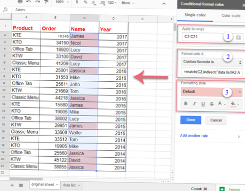
How do I conditional format based on another sheet in Google Sheets?

Highlight Cells Using Conditional Formatting Based on Another Cell Value in Google Sheets

1. Select the cells that have the names (A2:A11).
2. Go to the Format Tab.
3. Click on Conditional Formatting.
4. In the Conditional Formatting rules pane, select Single Color.
5. From the 'Format Cells if' drop down, select 'Custom Formula is'.

How do I link conditional formatting to another sheet?

Compare Cells on Two Sheets

1. Select cells A1:C8 on Sheet1, with A1 as the active cell.
2. On the Ribbon, click the Home tab, and click Conditional Formatting.
3. Click Highlight Cell Rules, then click Greater Than.
4. In the Greater Than dialog box, click in the cell reference box.
5. Click on the tab for Sheet2.

Can I conditional format a cell based on another?

When you want to format a cell based on the value of a different cell, for example to format a report row based on a single column's value, you can use the conditional formatting feature to create a formatting formula.

Can you apply conditional formatting to multiple sheets?

Re: Conditional formatting rules in multiple sheets

It is not possible to simultaneously apply conditional formatting to different columns in different sheet tab because when you group two or more sheets by using SHIFT key, the Conditional Formatting is greyed out... ... You can do this running on many sheets.

Does Google sheets have conditional formatting?

Create a conditional formatting rule

On your Android phone or tablet, open a spreadsheet in the Google Sheets app. Select the range you want to format. Conditional formatting. ... If there's already a rule in the cell or range, to add another, tap ADD first.

How do I conditional format a row based on one cell in Google Sheets?

To format an entire row based on the value of one of the cells in that row:

1. On your computer, open a spreadsheet in Google Sheets.
2. Select the range you want to format, for example, columns A:E.
3. Click Format Conditional formatting.
4. Under the "Format cells if" drop-down menu, click Custom formula is.

How do I apply the same format to all sheets in Excel?

As a recap – here's how to format multiple sheets at the same time:

1. Ctrl + Click each sheet tab at the bottom of your worksheet (selected sheets will turn white).
2. While selected, any formatting changes you make will happen in all of the selected sheets.
3. Double-click each tab when you are done to un-select them.

How do I automatically link a cell color to another sheet in Excel?

How to automatically link a cell color to another in Excel?

1. Right click the sheet tab you need to link a cell color to another, and then click View Code from the right-clicking menu.
2. In the opening Microsoft Visual Basic for Applications window, please copy and paste the below VBA code into the Code window.

How can I identify duplicates between two Excel sheets?

Select both columns of data that you want to compare. On the Home tab, in the Styles grouping, under the Conditional Formatting drop down choose Highlight Cells Rules, then Duplicate Values. On the Duplicate Values dialog box select the colors you want and click OK. Notice Unique is also a choice.

How do you conditional format a cell based on a date?

Excel conditional formatting for dates (built-in rules)

1. To apply the formatting, you simply go to the Home tab > Conditional Formatting > Highlight Cell Rules and select A Date Occurring.
2. Select one of the date options from the drop-down list in the left-hand part of the window, ranging from last month to next month.

How do I populate a cell in Excel based on another cell?

Fill data automatically in worksheet cells

1. Select one or more cells you want to use as a basis for filling additional cells. For a series like 1, 2, 3, 4, 5..., type 1 and 2 in the first two cells. For the series 2, 4, 6, 8..., type 2 and 4. ...
2. Drag the fill handle .
3. If needed, click Auto Fill Options. and choose the option you want.

Which formatting options can be set for conditional formatting rules?

Which formatting option(s) can be set for Conditional Formatting rules? Any of these formatting options as well as number, border, shading, and font formatting can be set.